Concave parsimony
Introduction
Some authors believed that parsimony and weithing were somehow mutually exclusive and parsimony analysis should use all characters with the same weight (Watrous and Wheeler,1981). Farris (1983) saw the relationship between parsimony and weighting, he showed the most parsimonious tree is the hypothesis with greatest explanatory power, given the weights of the characters. Several authors are in favor of character weighting and consider that characters with more homoplasy are less reliable. In other words weighting characters inversely to their homoplasy would improve the results (Goloboff, 1993). The method consist of searching trees with maximum total fit, this character fits are defined as a concave function of homoplasy. The fittest trees imply that have fewer steps for the characters which fit tree better. The weight of a character is a function of its fit to a tree. Therefore, the fit for each character would be measured as a function of its homoplasy and the total fit of the tree would be the sum of the fits of the characters (Goloboff, 1993).
Methodology
Simulate DNA sequences in Seq-gen (Rambaut and Grassly, 1997), with differents sequence lengths (10, 100 and 1000) under the evolutionary models GTR, F84 and HKY for each sequence length. Then, a parsimony analysis using implied weighting with differents values of concavity constant (K=1, K=10, K=40, K=100, and K=1000) implemented in TNT v.1.5 (Goloboff et al., 2001). To see the difference between implied weight and unweight carried out another parsimony analysis without implied weighting. To explore the sensitivity of topology under differents weights and unweights carried out the Robinson-Foulds metric or symmetric difference (Robinson & Foulds, 1981) in software R v 3.2.3 (R Core Team, 2014) and also to compare the reference tree (simulated under Farris and Felsenstein zone) with implied weights and unweights.
Results and discussion
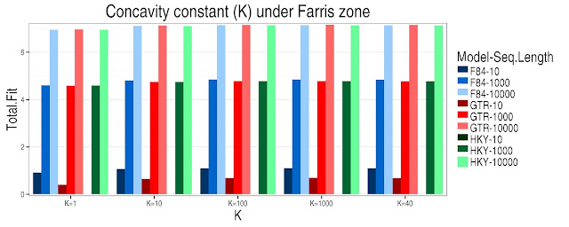
In the Felsenstein and Farris zone can be seen that under the same model and the same sequence length there is an increase in the value of Total Fit as it increases the value of concavity constant (K). In general as the sequence length increases under the same model there is an increases in the Total Fit. In the Felsenstein zone is noted that under the model GTR-10 the Total Fit is zero with differents K values, for models F84 -10 y HKY-10 have a Total Fit of 1 under differents K values. The highest Total Fit values are under the model F84-10000 (Fig 1). In the Farris zone the models with the smallest sequence lengths have the lowest Total Fit values and these in turn decrease as the K value decreases and the models with longest sequence length have the highest Total Fit values as the K value increases (Fig 2).
The K values didn't have influence over the topology under the same model and the same sequence length. In other words it recovered the same topology under the same model with the same sequence length. For that reason I applied the Robinson Foulds metric among a tree for each model and sequence length with implied weights and one for unweight. In the Felsenstein zone with implied weights vs unweight it recovered the same topology (RF=0) for all models except for GTR-10 model (RF=2) (Fig 3). In the Farris zone F84-1000, GTR-1000 and HKY-1000 models recovered the same topology.
RF metric for tree reference vs implied weights showed that in the Farris zone recovered the most of topologies except for F84-10 and GTR-10 and non-weights recovered the same topologies except fot F84-10. In contrast for Felsenstein zone with implied weights recovered the same topology under GTR1000 and HKY-1000 and non-weights recovered F84-1000, GTR1000 and HKY-1000 (Fig 4, 5).
In conclusion, the homoplasy can be related to how long is the sequence length and the nucleotide substitution model to use, but not only this, I think it also depends on how conservative is the nucleotidic sequence.
Figure 1. Felsenstein zone. The Total Fit values for each concavity constant (K), under different models and sequence length, the total fit was transformed with natural logarithm for a better comparison. Models GTR-10000, F84-10000 y HKY-10000 have highest Total Fit values.
Figure 2. Farris zone. The Total Fit values for each concavity constant (K), under different models and sequence length, the total fit was transformed with natural logarithm for a better comparison. Under the HKY model and sequence length of 10 the K value is 1 (log(1)=0).
Figure 3. Robinson-Foulds metric (RF) for the Felsenstein and Farris zone (implied weights vs unweights).
Figure 4-5. RF metric among Farris and Felsenstein zones (weight-unweight) with tree reference.
Bibliography
Goloboff, P. A., Farris, J. S., & Nixon, K. C. (2008). TNT, a free program for phylogenetic analysis. Cladistics, 24(5), 774-786.
Felsenstein, J. (1978). Cases in which parsimony or compatibility methods will be positively misleading. Systematic Biology, 27(4), 401–410.
Goloboff, P., 1993. Estimating character weights during tree search. Cladistics 9, 83–91.
Goloboff, P., 1997. Self-weighted optimization: tree searches and character state reconstructions under implied transformation costs. Cladistics 13, 225–245.
Goloboff, P., 2013. Extended implied weighting. Cladstics 1-13.
Robinson, D., & Foulds, L. R. (1981). Comparison of phylogenetic trees. Mathematical Biosciences, 53(1), 131–147.
R Core Team. (2014). R: A Language and Environment for Statistical Computing. Vienna, Austria.
Watrous, L. and Q. Wheeler. 1981. The out-group compariso method of character analysis. Syst. Zool. 30:1-11.


No hay comentarios:
Publicar un comentario